
Gigabyte GA-7PESH1 Review: A Dual Processor Motherboard through a Scientist’s Eyes
- Posted in
- Motherboards
- Gigabyte
- C602
Two Dimensional Implicit Finite Difference
The ‘Finite Difference’ part of this computational grid solver means that the derivation of this method is similar to that shown in the Explicit Finite Difference method on the previous page. We are presented with the following equation which explains Fick’s first law of diffusion for mass transport in three dimensions:
 [8]
The implicit method takes the view that the concentrations at time t+1 are a series of unknowns, and the equations are thus coupled into a series of simultaneous equations with an equal set of unknowns, which must be solved together:
 [9]
 [10]
The implicit method is algorithmically more complex than the explicit method, but does offer the advantage of unconditional stability with respect to time.
The Alternating Direction Implicit (ADI) Method
For a system in two dimensions (labelled r and z), such as a microdisk simulation, the linear system has to be solved in both directions using Fick’s Laws:

 [11]
The alternating direction implicit (ADI) method is a straightforward solution to solving what are essentially two dimensional simultaneous equations whilst retaining a high degree of algorithm stability.
ADI splits equation [11] into two half time steps – by treating one dimension explicitly and the other dimension implicitly in the same half time step. Thus the explicit values known in one direction are fed into the series of simultaneous equations to solve the other direction. For example, using the r direction explicitly to solve the z direction implicitly:
 [12]
 [13]
By solving equation [13] for the concentrations in the z direction, the next half time step concentrations can be calculated for the r direction, and so on until the desired time in simulation is achieved. These time step equations are solved using the Thomas Algorithm for tri-diagonal matrices.
Application to this Review
For the purposes of this review, we generate an x-by-x grid of points with a relative concentration of 1, where the boundaries are fixed at a relative concentration of 0. The grid is a regular grid, simplifying calculations. The nature of the simulation allows that for each half-time step to focus on calculating in one dimension, for a simulation of x-by-x nodes we can spawn x threads as adjacent rows/columns (depending on direction) are independent. These threads, in comparison to the explicit finite difference, are substantially bulkier in terms of memory usage.
The code was written in Visual Studio C++ 2012 with OpenMP as the multithreaded source. The main function to do the calculations is as follows.
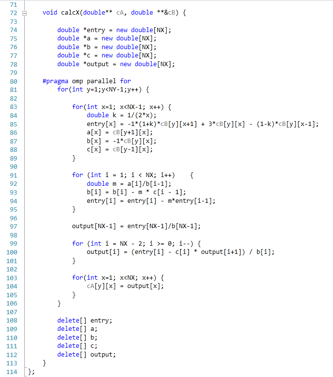
For our scores, we increase the size of the grid from a 2x2 until we hit 2GB memory usage. At each stage, the time taken to repeatedly process the grid over many time steps is calculated in terms of ‘million nodes per second’, and the peak value is used for our results.
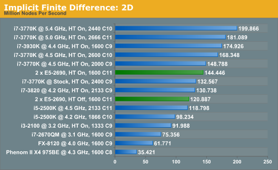
Previously where the explicit 2D method was indifferent to HyperThreading and the explicit 3D method was very sensitive; the implicit 2D is a mix of both. There are still benefits to be had from enabling HyperThreading. Nevertheless, the line between single processor systems and dual processors is being blurred a little due to the different speeds of the SP results, but in terms of price/performance, the DP system is at the wrong end.
Originally published at https://www.anandtech.com/show/6533/gigabyte-ga7pesh1-review-a-dual-processor-motherboard-through-a-scientists-eyes (Wayback Machine).