
Gigabyte GA-7PESH1 Review: A Dual Processor Motherboard through a Scientist’s Eyes
- Posted in
- Motherboards
- Gigabyte
- C602
Explicit Finite Difference
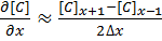
For a grid of points or nodes over a simulation space, each point in the space can describe a number of factors relating to the simulation – concentration, electric field, temperature, and so on. In terms of concentration, the material balance gradients are approximated to the differences in the concentrations of surrounding points. Consider the concentration gradient of species C at point x in one dimension, where [C]x describes the concentration of C at x:
 [1]
The second derivative around point x is determined by combining the half-differences from the adjacent half-points next to x:
 [2]
Equations [1] and [2] can be applied to the partial differential equation [3] below to reveal a set of linear equations which can be solved.
Fick’s first law for the rate of diffusional mass transport can be applied in three dimensions:
 [3]
where D is the diffusion coefficient of the chemical species, and t is the time. For the dimensional analyses used in this work, the Laplacian is split over the Cartesian dimensions x, y and z.
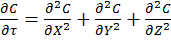
Dimension transformations are often employed to these simulations to relieve the simulation against scaling factors. The expansion of equation [3] given specific dimension transforms not mentioned here give equation [4] to be solved.
 [4]
The expansion of equation [4] using coefficient collation and expansion by finite differences mentioned in equations [1] and [2] lead to equation [5]:

 [5]
Equation [5] represents a series of concentrations that can be calculated independently from each other – each concentration can now be solved for each timestep (t) by an explicit algorithm for t+1 from t.
The explicit algorithm is uncommonly used in electrochemical simulation, often due to stability constraints and time taken to simulate. However, it offers complete parallelisation and low thread density – ideal for multi-processor systems and graphics cards – such that these issues should be overcome.
The explicit algorithm is stable when, for equation [4], the Courant–Friedrichs–Lewy condition [6] holds.
 [6]
Thus the upper bound on the time step is fixed given the minimum grid spacing used.
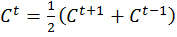
There are variations of the explicit algorithm to improve this stability, such as the Dufort-Frankel method of considering the concentration at each point as the linear function of time, such that:
 [7]
However, this method requires knowledge of the concentrations of two steps before the current step, therefore doubling memory usage.
Application to this Review
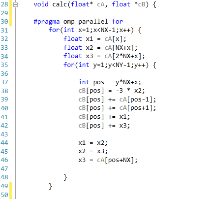
For the purposes of this review, we generate an x-by-x / x-by-x-by-x grid of points with a relative concentration of 1, where the boundaries are fixed at a relative concentration of 0. The grid is a regular grid, simplifying calculations. As each node in the grid is independently calculable from each other, it would be ideal to spawn as many threads as there are nodes. However, each node has to load the data of the nodes of the previous time step around it, thus we restrict parallelization in one dimension and use an iterative loop to restrict memory loading and increase simulation throughput.
The code was written in Visual Studio C++ 2012 with OpenMP as the multithreaded source. The main functions to do the calculations are as follows.
For 2D:
For 3D:
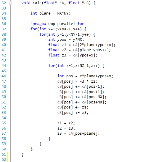
For our scores, we increase the size of the grid from a 2x2 or 2x2x2 until we hit 2GB memory usage. At each stage, the time taken to repeatedly process the grid over many time steps is calculated in terms of ‘million nodes per second’, and the peak value is used for our results.
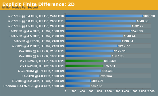
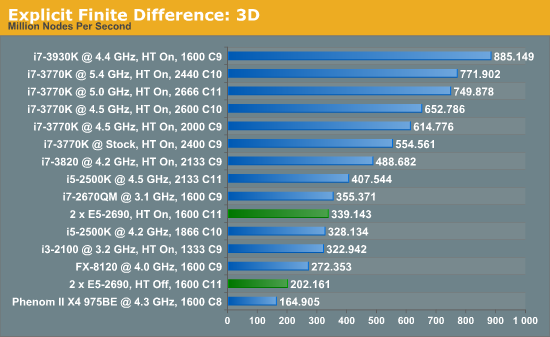
Firstly, the results for our 2D and 3D Explicit Finite Difference simulations are shocking. In 3D, the dual processor system gets beaten by a mobile i7-2670QM (!). In both 2D and 3D, it seems being able to quickly access main memory and L3 caches is top priority. Each processor in the DP machine has to go out to memory when they need a value not in cache, whereas in a single processor machine it can access the L3 cache if the simulation fits wholly in there and the processor can predict which numbers are required next.
Also it should be noted that enabling HyperThreading in 3D gave a better than 50% increase in throughput on the dual processor machine.
Originally published at https://www.anandtech.com/show/6533/gigabyte-ga7pesh1-review-a-dual-processor-motherboard-through-a-scientists-eyes (Wayback Machine).